Volume Rendering in Unity
Volume Rendering in Unity
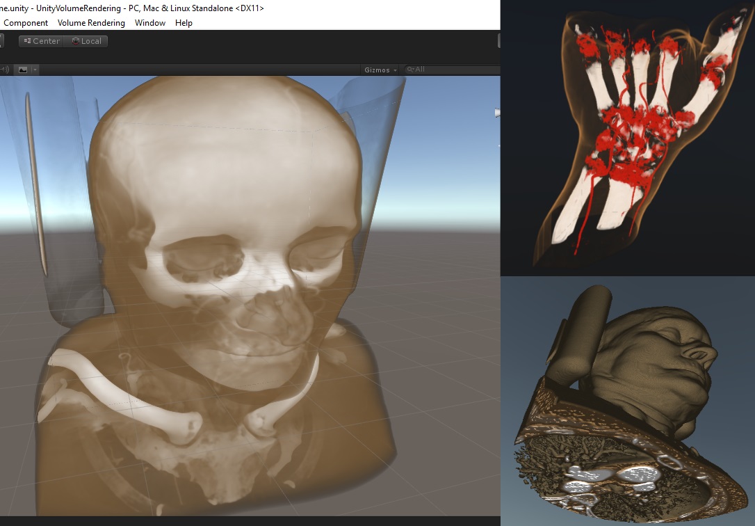
In this article I will explain how volume rendering can be implemented in Unity. I will use one of my hobby projects as an example: https://github.com/mlavik1/UnityVolumeRendering
If you are not familiar with shaders in Unity (or shaders in general), you might want to study that first. You could also read my slides about shaders in Unity: https://www.slideshare.net/MatiasLavik/shaders-in-unity Volume Rendering
First of all, what is volume rendering? Wikipedia describes volume rendering as “a set of techniques used to display a 2D projection of a 3D discretely sampled data set”. There are many use cases for volume rendering, but one of them is visualisation of CT scans. If you break your leg the doctor might take a CT scan of your leg. The scan produces a 3-dimensional dataset, where each cell defines the density at that point.
The data:
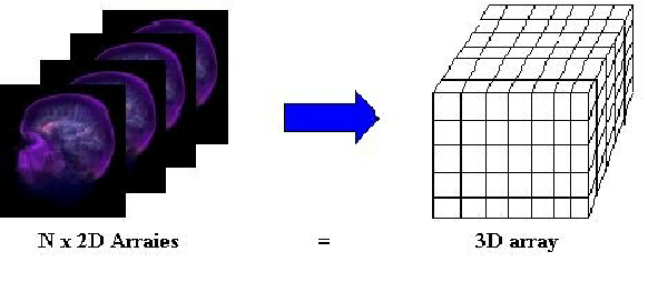
- We use 3D voxel data from a medical CT scan.
- The value of each data point represents the density at that point.
- The data is read from a file and stored in a 3D texture
- The data fits nicely into a box, so we render a box (we only draw the back faces) and use raymarching to fetch the densities of each visible voxel inside the box.
 ([illustration by: Klaus D Tönnies](https://www.researchgate.net/figure/3D-volume-data-representation_fig1_238687132))
This data can then be rendered in 3D using volume rendering.

This is done using a technique called “raymarching”.
Raymarching
Raymarching is a technique similar to raytracing, except instead of finding intersections you move along the ray at even (or un-even) steps and collect values.
Raytracing: Cast a ray from the eye through each pixel and find the first triangle(s) hit by the ray. Then draw the colour of that triangle . Usage: Rendering triangular 3D models (discrete)
Raymarching: Create a ray from/towards the camera. Divide the ray into N steps/samples, and combine the value at each step. Usage: Rendering continous data, such as mathematical equations. Rendering volume data (such as CT scans)
For CT scans we want to see both the skin, blood veins and bones at the same time – ideally with different colours
Implementation:
- Draw the back-faces of a box
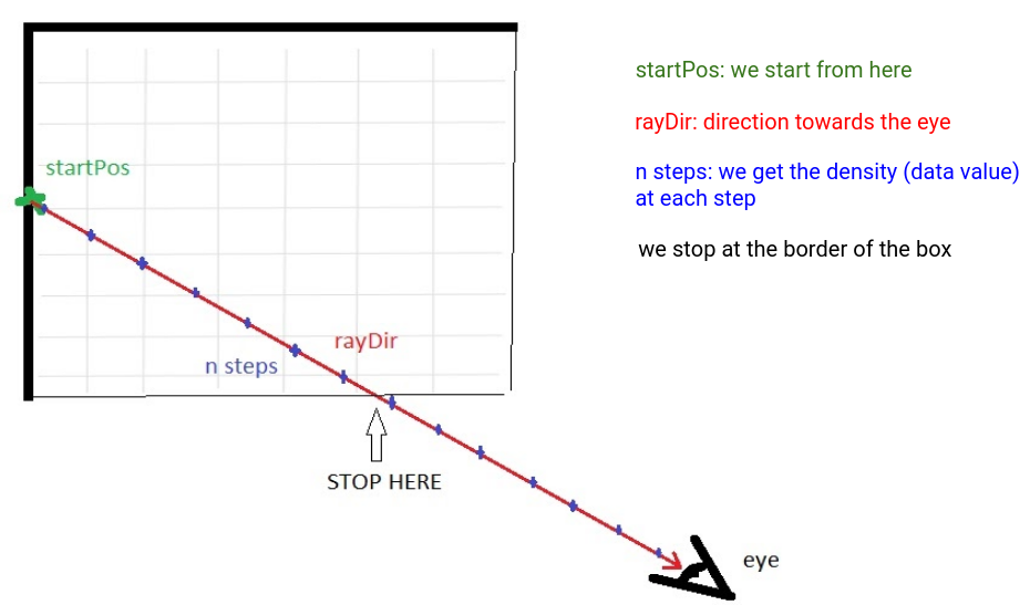
- For each vertex:
- Set startPos as the vertex local position
- Set rayDir as the direction towards the eye (in model space)
- Divide the ray into N steps/samples
- For each step (starting at startPos moving along rayDir)
- Get the density: use currentPos as a texture coordinate and fetch the value from the 3D texture
- ??? (use the density to decide the output colour of the fragment/pixel)
The code:
// Direct Volume Rendering
fixed4 frag_dvr (v2f i)
{
#define NUM_STEPS 512
    const float stepSize = 1.732f/*greatest distance in box*/ / NUM_STEPS;

    float3 rayStartPos = i.vertexLocal + float3(0.5f, 0.5f, 0.5f);
    float3 rayDir = normalize(ObjSpaceViewDir(float4(i.vertexLocal, 0.0f)));

    float4 col = float4(0.0f, 0.0f, 0.0f, 0.0f);
    for (uint iStep = 0; iStep < NUM_STEPS; iStep++)
    {
        const float t = iStep * stepSize;
        const float3 currPos = rayStartPos + rayDir * t;
        if (currPos.x < 0.0f || currPos.x >= 1.0f || currPos.y < 0.0f || currPos.y > 1.0f || currPos.z < 0.0f || currPos.z > 1.0f) // TODO: avoid branch?
            break;

        const float density = getDensity(currPos);

        // TODO: modify "col" based on the density
    }
    return col;
}
Next, let’s look at some techniques for determining the output colour. We will look at 3 techniques:
- Maximum intensity projection
- Direct volume rendering
- Isosurface rendering
1. Maximum Intensity Projection
This is the simplest of the three techniques. Here we simply draw the voxel (data value) with the highest density along the ray. The output colour will be white, with alpha = maxDensity.
This is a simple but powerful visualisation, that highlights bones and big variations in density.
fixed4 frag_mip(v2f i)
{
#define NUM_STEPS 512
const float stepSize = 1.732f/*greatest distance in box*/ / NUM_STEPS;
float3 rayStartPos = i.vertexLocal + float3(0.5f, 0.5f, 0.5f);
float3 rayDir = normalize(ObjSpaceViewDir(float4(i.vertexLocal, 0.0f)));
float maxDensity = 0.0f;
for (uint iStep = 0; iStep < NUM_STEPS; iStep++)
{
const float t = iStep * stepSize;
const float3 currPos = rayStartPos + rayDir * t;
// Stop when we are outside the box
if (currPos.x < 0.0f || currPos.x >= 1.0f || currPos.y < 0.0f || currPos.y > 1.0f || currPos.z < 0.0f || currPos.z > 1.0f)
break;
const float density = getDensity(currPos);
if (density > _MinVal && density < _MaxVal)
maxDensity = max(density, maxDensity);
}
// Maximum intensity projection
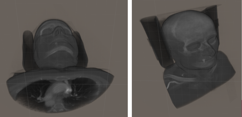
float4 col = float4(1.0f, 1.0f, 1.0f, maxDensity);
return col;
}
And this is the result:
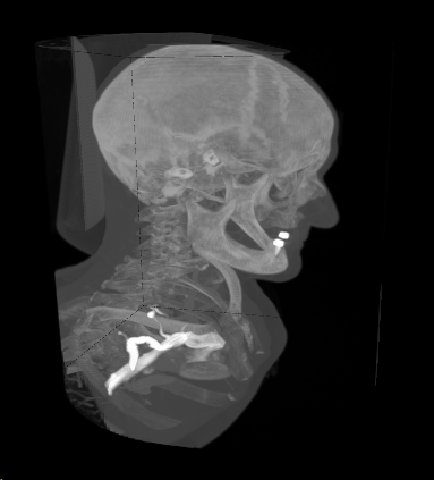
2. Direct Volume Rendering with compositing
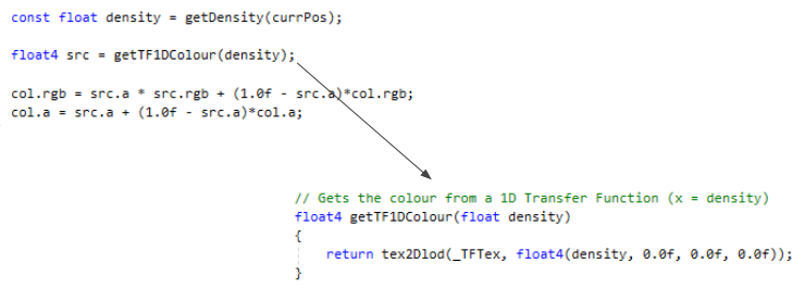
This is probably the most advanced of the thress techniques. However the basic idea is this: On each step, combine the current voxel colour with the accumulated colour value from the previous steps.
We linearly interpolate the RGB values, like this: newRGB = lerp(oldRGB, currRGB, currAlpha). And then add the new alpha to the old alpha multiplied by (1 – new alpha).
col.rgb = src.a * src.rgb + (1.0f – src.a)*col.rgb;
col.a = src.a + (1.0f – src.a)*col.a;
Full shader code:
// Direct Volume Rendering
fixed4 frag_dvr (v2f i)
{
#define NUM_STEPS 512
    const float stepSize = 1.732f/*greatest distance in box*/ / NUM_STEPS;

    float3 rayStartPos = i.vertexLocal + float3(0.5f, 0.5f, 0.5f);
    float3 rayDir = normalize(ObjSpaceViewDir(float4(i.vertexLocal, 0.0f)));

    float4 col = float4(0.0f, 0.0f, 0.0f, 0.0f);
    for (uint iStep = 0; iStep < NUM_STEPS; iStep++)
    {
        const float t = iStep * stepSize;
        const float3 currPos = rayStartPos + rayDir * t;
        if (currPos.x < 0.0f || currPos.x >= 1.0f || currPos.y < 0.0f || currPos.y > 1.0f || currPos.z < 0.0f || currPos.z > 1.0f) // TODO: avoid branch?
            break;

        const float density = getDensity(currPos);

        float4 src = float4(density, density, density, desntiy * 0.1f);

        col.rgb = src.a * src.rgb + (1.0f - src.a)*col.rgb;
        col.a = src.a + (1.0f - src.a)*col.a;

        if(col.a > 1.0f)
            break;
    }
    return col;
}
And the results:
But we are not done yet! We can get much more interesting visualisations by adding colour and filtering using a transfer function. We’ll come back to this soon!
3. Isosurface Rendering
The most basic implementation of isosurface rendering is quite simple: Draw the first voxel (data value) with a density higher than some threshold.
Now we need to start raymarching at the eye (or ideally at the point where the ray hits the front face of the box) and move away from the eye. When we hit a voxel with density > threshold we stop, and use that density.
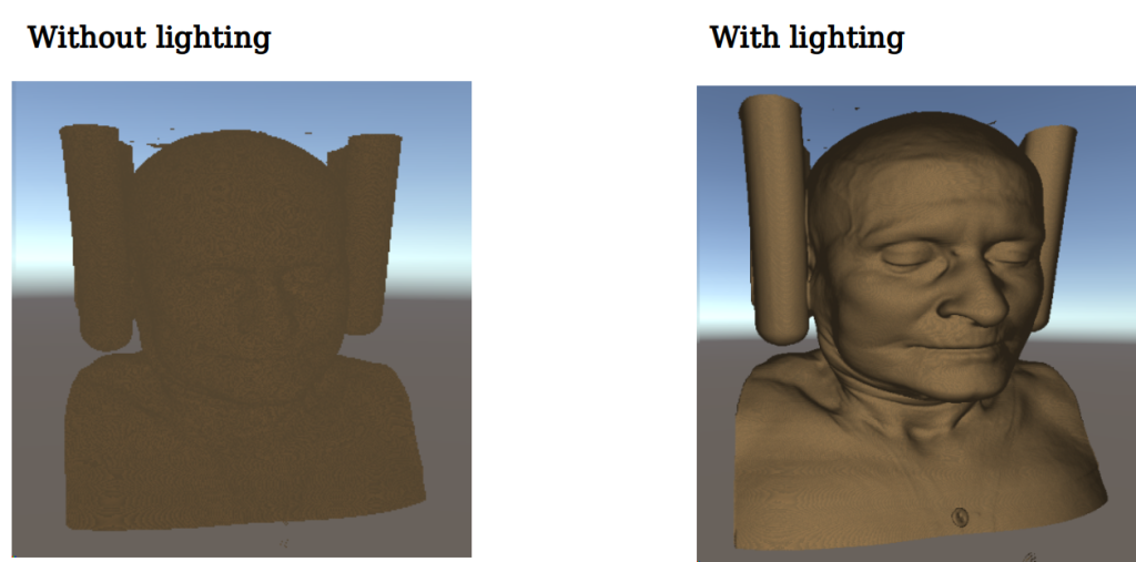
This is simple to implement, but if you try it you might be disappointed by how bad the result looks. However, if we add some lighting it will look a lot better. Lighting
Since we are rendering the surfaces only, we need light reflection to make it look good. For our example we will only use “diffuse” reflection.
Diffuse reflection:
Light intensity is decided by the angle between the direction to the light source and the surface normal (θ), and a diffuse constant (Kd – we can set it to 1).
Id = Kd · cos(θ)
When l and n are normalised, we have:
cos(θ) = dot(n, l)
This gives us:
Id = Kd · dot(n, l)
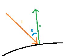
How do we get the normal?
Since we are working with 3D voxels and not triangles, getting the normal requires some extra work.
Solution: Use the gradient
The gradient is simply the direction of change. If the density increases/decreases in a certain direction, that direction is the gradient – our normal.
Compare the neighbour data values in each axis:
float xDiff = data[x-1, y, z] - data[x+1, y, z;]
float yDiff = data[x, y-1, z] - data[x, y+1, z;]
float zDiff = data[x, y, z-1] - data[x, y, z+1;]
float3 gradient = float3(xDiff, yDirr, zDiff)
float3 normal = normalize(gradient);
As you see from the above code: when the data values decrease towards the right (positive X-axis), the normal will point to the right.
fixed4 frag_surf(v2f i)
{
#define NUM_STEPS 1024
    const float stepSize = 1.732f/*greatest distance in box*/ / NUM_STEPS;

    float3 rayStartPos = i.vertexLocal + float3(0.5f, 0.5f, 0.5f);
    float3 rayDir = normalize(ObjSpaceViewDir(float4(i.vertexLocal, 0.0f)));
    // Start from the end, tand trace towards the vertex
    rayStartPos += rayDir * stepSize * NUM_STEPS;
    rayDir = -rayDir;

    float3 lightDir = -rayDir;

    // Create a small random offset in order to remove artifacts
    rayStartPos = rayStartPos + (2.0f * rayDir / NUM_STEPS) * tex2D(_NoiseTex, float2(i.uv.x, i.uv.y)).r;

    float4 col = float4(0,0,0,0);
    for (uint iStep = 0; iStep < NUM_STEPS; iStep++)
    {
        const float t = iStep * stepSize;
        const float3 currPos = rayStartPos + rayDir * t;
        // Make sure we are inside the box
        if (currPos.x < 0.0f || currPos.x >= 1.0f || currPos.y < 0.0f || currPos.y > 1.0f || currPos.z < 0.0f || currPos.z > 1.0f) // TODO: avoid branch?
            continue;

        const float density = getDensity(currPos);
        if (density > _MinVal && density < _MaxVal)
        {
            float3 normal = normalize(getGradient(currPos));
            float lightReflection = dot(normal, lightDir);
            lightReflection =  max(lerp(0.0f, 1.5f, lightReflection), 0.5f);
            col = lightReflection * getTF1DColour(density);
            col.a = 1.0f;
            break;
        }
    }

    return col;
}
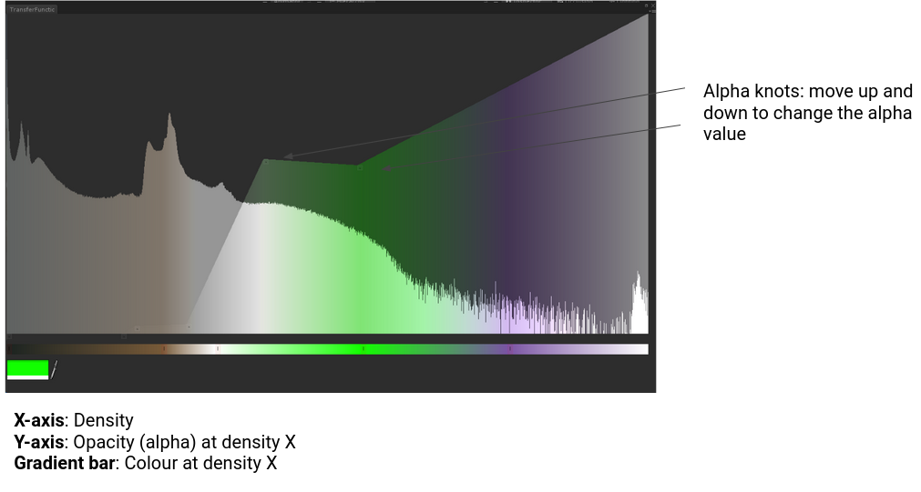
Transfer Functions
Basic idea: Use the density to decide colour and opacity/transparency.
Example:
- Bones (high density) are white and opaque
- Blood vessels are red and semi-transparent
- The skin (low density) is brown and almost invisible
Implementation:
- Allow the user to add colour knots and alpha knots to a graph, where the x-axis represents the density and the y-axis defines the opacity
- Generate a 1D texture where x-axis = density and the textel (pixel)’s RGBA defines the colour and opacity.
- Shader: After getting the density of a voxel, use the density to look up the RGBA value in the transfer function texture.
 Note: Unity doesn’t support 1D textures so we use a 2D texture with height=1
And here is the updated shader code (almost the same as before, except the colour now comes from the transfer function):
float4 getTF1DColour(float density)
{
    return tex2Dlod(_TFTex, float4(density, 0.0f, 0.0f, 0.0f));
}

// Direct Volume Rendering
fixed4 frag_dvr (v2f i)
{
#define NUM_STEPS 512
    const float stepSize = 1.732f/*greatest distance in box*/ / NUM_STEPS;

    float3 rayStartPos = i.vertexLocal + float3(0.5f, 0.5f, 0.5f);
    float3 rayDir = normalize(ObjSpaceViewDir(float4(i.vertexLocal, 0.0f)));

    float4 col = float4(0.0f, 0.0f, 0.0f, 0.0f);
    for (uint iStep = 0; iStep < NUM_STEPS; iStep++)
    {
        const float t = iStep * stepSize;
        const float3 currPos = rayStartPos + rayDir * t;
        if (currPos.x < 0.0f || currPos.x >= 1.0f || currPos.y < 0.0f || currPos.y > 1.0f || currPos.z < 0.0f || currPos.z > 1.0f) // TODO: avoid branch?
            break;

        const float density = getDensity(currPos);

        float4 src = getTF1DColour(density);

        col.rgb = src.a * src.rgb + (1.0f - src.a)*col.rgb;
        col.a = src.a + (1.0f - src.a)*col.a;

        if(col.a > 1.0f)
            break;
    }
    return col;
}
This is the result:
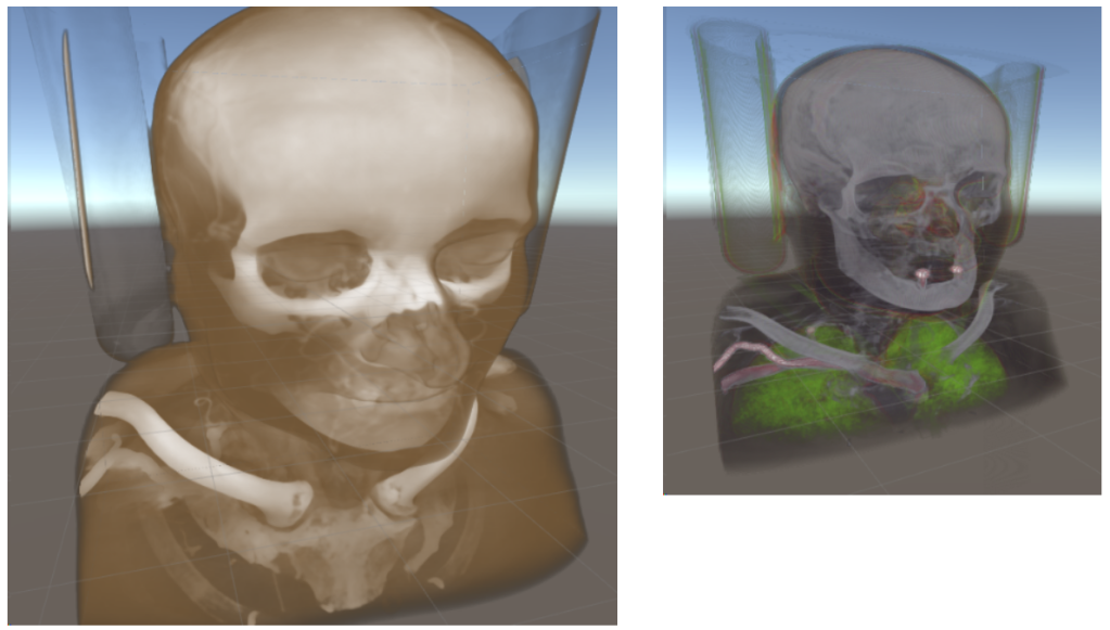
For the transfer function texture creation, see: https://github.com/mlavik1/UnityVolumeRendering/blob/master/Assets/Scripts/TransferFunction/TransferFunction.cs
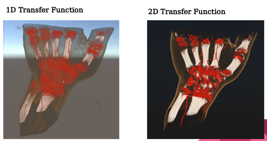
Multidimensional Transfer Functions
Sometimes opacity is not enough to identify the parts we want to highlight. Different parts of the dataset might have similar densities. So ideally we need another dimension in our transfer function.
Gradient magnitude:
- Gradient = direction of change (already covered this in previous slides)
- Gradient magnitude = magnitude (length) of the gradient vector (= how much the density changes at the point – or the “derivative” if you want)
Using both density and gradient magnitude when setting colours/alphas allows us to highlight surfaces while ignoring what’s beneath it. For example, the skin has a relatively low density, but other parts of the body might also have similar desity. However, the skin also has another distinctive feature: since the skin is the outermost layer on the human body it also has a relatively large gradient magnitudy (compared to its density). Using both density and gradient magnitude we can more easily identify the skin in the dataset.
We first add two new helper functions:
// Gets the gradient at the specified position
float3 getGradient(float3 pos)
{
    return tex3Dlod(_DataTex, float4(pos.x, pos.y, pos.z, 0.0f)).rgb;
}

// Gets the colour from a 2D Transfer Function (x = density, y = gradient magnitude)
float4 getTF2DColour(float density, float gradientMagnitude)
{
    return tex2Dlod(_TFTex, float4(density, gradientMagnitude, 0.0f, 0.0f));
}
We then use these in the main shader, to set the colour (“src”):
float3 gradient = getGradient(currPos);
float mag = length(gradient) / 1.75f;
float4 src = getTF2DColour(density, mag);
Results:
This is how GUI for creating 2D transfer functions look:
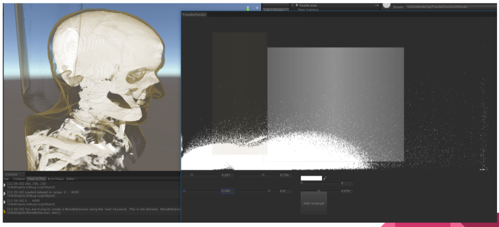
X-axis = density Y-axis = gradient magnitude
This might be a little bit hard to digest at first, but we use boxes to create the transfer functions. The area covered by the box defines the selection the of density values and gradient magnitude values that we want to map to a certain colour. The colour of the box defines the colour of the selected density/gradient magnitude values, and we also set a minimum and maximum alpha (max at the box centre, and min at the border).
Only using boxes might not be sufficient, so ideally we should also support other shapes.
For more info (and description of 2D transfer function GUI) see Multi-Dimensional Transfer Functions for Volume Rendering (Kniss et al.).
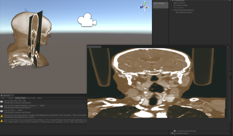
Slice rendering
Another much used volume rendering technique is slice rendering. This is basically a 2D visualisation of the dataset, where we render a single slice of the model.
Implementation:
- Create a movable plane
- In the shader, use the plane’s vertex coordinates (relative to the volume model) as texture coordinates for the volume data (which is a 3D texture).
- (optionally) use 1D transfer function to apply colour
fixed4 frag (v2f i) : SV_Target
{
    float3 dataCoord = i.relVert +float3(0.5f, 0.5f, 0.5f);
    float dataVal = tex3D(_DataTex, dataCoord).a;
    float4 col = tex2D(_TFTex, float2(dataVal, 0.0f));
    col.a = 1.0f;

    return col;
}
For the whole shader, see: https://github.com/mlavik1/UnityVolumeRendering/blob/master/Assets/Shaders/SliceRenderingShader.shader
Notes on shaders in Unity
Unity uses its own shader language (based on CG). The shaders are automatically converted to HLSL/GLSL, but Unity have added several nice features on top of this!
#pragma multi_compile
The first 3 techniques (direct volume rendering, maximum intensity project, isosurface rendering) use mostly the same input data. It could be convenient to combine all of them in one shader, using different models. Unity allows us to do this through #pragma multi_compile.
We can define 3 rendering modes like this: 1
#pragma multi_compile MODE_DVR MODE_MIP MODE_SURF
We add this to the shader pass, just after “CGPROGRAM” (see the example shader). This will make Unity create 3 versions of the shader: One with MODE_DVR defines, one with MODE_MIP defined and one with MODE_SURF defined. We can then use #if to check (at “compile” time) which mode we are using, like this:
fixed4 frag(v2f i) : SV_Target
{
#if MODE_DVR
    return frag_dvr(i);
#elif MODE_MIP
    return frag_mip(i);
#elif MODE_SURF
    return frag_surf(i);
#endif
}
Loop unrolling
Loops in shaders can be very expensive. However, by adding the “[unroll]” keyword before a loop you can “unroll” loops. This will create a linear “unrolled” version of the loop, which is faster to execute. However, it will increase the shader compilation time, and there is a maximum loop count.
Example:
for (x = 0; x < 3; x++)
    doSomething(x);
will become:
doSomething(0);
doSomething(1);
doSomething(2);
Read more about loop unrolling here.
References / credits
ImageVis3D:
- Some of the GUIs are heavily inspired by ImageVis3D
- Get ImageVis3D here: http://www.sci.utah.edu/software/imagevis3d.html
Marcelo Lima:
- Marcelo presented his implementation of isosurface rendering during his assignment presentation for the Visualisation course at the University of Bergen.
- See his amazing project here: https://github.com/m-lima/KATscans
Sharing is caring!